Create a PivotTable to analyze worksheet data

A PivotTable is a powerful tool to calculate, summarize, and analyze data that lets you see comparisons, patterns, and trends in your data. PivotTables work a little bit differently depending on what platform you are using to run Excel.

1. Select the cells you want to create a PivotTable from.

Note: Your data should be organized in columns with a single header row. See the Data format tips and tricks section for more details.

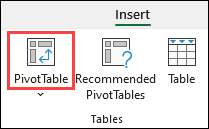
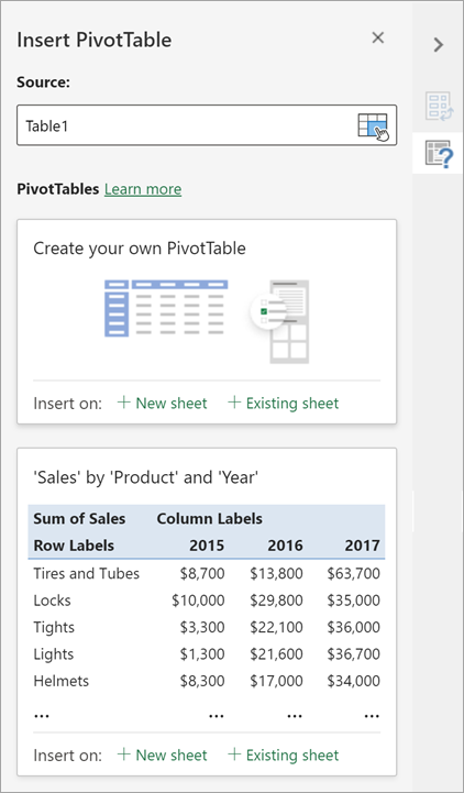
Select Insert >PivotTable.

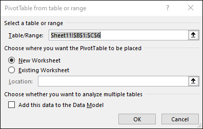
This creates a PivotTable based on an existing table or range.

Note: Selecting Add this data to the Data Model adds the table or range being used for this PivotTable into the workbook’s Data Model. Learn more.

By clicking the down arrow on the button, you can select from other possible sources for your PivotTable. In addition to using an existing table or range, there are three other sources you can select from to populate your PivotTable.

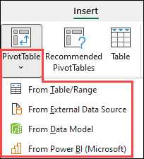
Note: Depending on your organization's IT settings you might see your organization's name included in the list. For example, "From Power BI (Microsoft)."

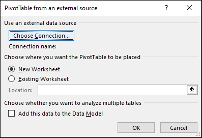
Get from External Data Source

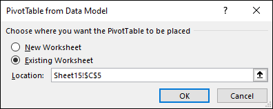
Get from Data Model

Use this option if your workbook contains a Data Model, and you want to create a PivotTable from multiple tables, enhance the PivotTable with custom measures, or are working with very large datasets.

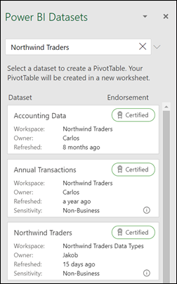
Get from Power BI

Use this option if your organization uses Power BI and you want to discover and connect to endorsed cloud datasets you have access to.

1. To add a field to your PivotTable, select the field name checkbox in the PivotTables Fields pane.

Note: Selected fields are added to their default areas: non-numeric fields are added to Rows, date and time hierarchies are added to Columns, and numeric fields are added to Values.

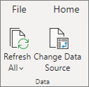
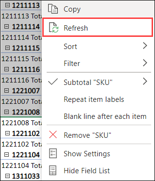
If you add new data to your PivotTable data source, any PivotTables that were built on that data source need to be refreshed. To refresh just one PivotTable, you can right-click anywhere in the PivotTable range, and then select Refresh. If you have multiple PivotTables, first select any cell in any PivotTable, then on the ribbon go to PivotTable Analyze > select the arrow under the Refresh button, and then select Refresh All.

Summarize Values By

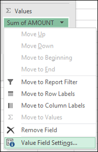
By default, PivotTable fields placed in the Values area are displayed as a SUM. If Excel interprets your data as text, the data is displayed as a COUNT. This is why it's so important to make sure you don't mix data types for value fields. You can change the default calculation by first selecting the arrow to the right of the field name, and then select the Value Field Settings option.

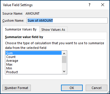
Next, change the calculation in the Summarize Values By section. Note that when you change the calculation method, Excel automatically appends it in the Custom Name section, like "Sum of FieldName", but you can change it. If you select Number Format, you can change the number format for the entire field.

Tip: Since changing the calculation in the Summarize Values By section changes the PivotTable field name, it's best not to rename your PivotTable fields until you're finished setting up your PivotTable. One trick is to use Find & Replace (Ctrl+H) >Find what > "Sum of", and then Replace with > leave blank to replace everything at once instead of manually retyping.

Show Values As

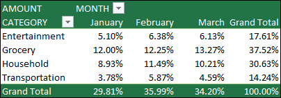
Instead of using a calculation to summarize the data, you can also display it as a percentage of a field. In the following example, we changed our household expense amounts to display as a % of Grand Total instead of the sum of the values.

Once you've opened the Value Field Setting dialog box, you can make your selections from the Show Values As tab.

Display a value as both a calculation and percentage.

Simply drag the item into the Values section twice, and then set the Summarize Values By and Show Values As options for each one.

1. Select a table or range of data in your sheet and select Insert > PivotTable to open the Insert PivotTable pane.
2. You can either manually create your own PivotTable or choose a recommended PivotTable to be created for you. Do one of the following:

• On the Create your own PivotTable card, select either New sheet or Existing sheet to choose the destination of the PivotTable.
• On a recommended PivotTable, select either New sheet or Existing sheet to choose the destination of the PivotTable.

Note: Recommended PivotTables are available only to Microsoft 365 subscribers.

You can change the data sourcefor the PivotTable data as you are creating it.

1. In the Insert PivotTable pane, select the text box under Source. While changing the Source, cards in the pane won't be available.
2. Make a selection of data on the grid or enter a range in the text box.
3. Press Enter on your keyboard or the button to confirm your selection. The pane updates with new recommended PivotTables based on the new source of data.

change the Destination." />

Get from Power BI

Use this option if your organization uses Power BI and you want to discover and connect to endorsed cloud datasets you have access to.

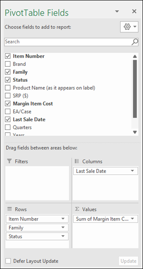
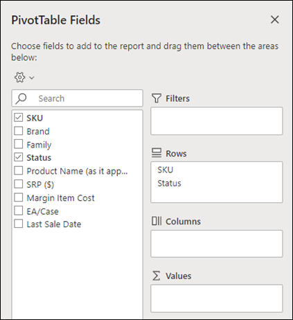
In the PivotTable Fields pane, select the check box for any field you want to add to your PivotTable.

By default, non-numeric fields are added to the Rows area, date and time fields are added to the Columns area, and numeric fields are added to the Values area.

You can also manually drag-and-drop any available item into any of the PivotTable fields, or if you no longer want an item in your PivotTable, drag it out from the list or uncheck it.

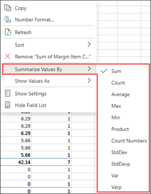
Summarize Values By

By default, PivotTable fields in the Values area are displayed as a SUM. If Excel interprets your data as text, it is displayed as a COUNT. This is why it's so important to make sure you don't mix data types for value fields.

Change the default calculation by right-clicking any value in the row and selecting the Summarize Values By option.

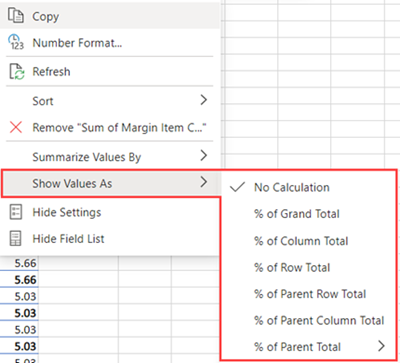
Show Values As

Instead of using a calculation to summarize the data, you can also display it as a percentage of a field. In the following example, we changed our household expense amounts to display as a % of Grand Total instead of the sum of the values.

Right-click any value in the column you'd like to show the value for. Select Show Values As in the menu. A list of available values displays.

Make your selection from the list.

To show as a % of Parent Total, hover over that item in the list and select the parent field you want to use as the basis of the calculation.

If you add new data to your PivotTable data source, any PivotTables built on that data source must be refreshed. Right-click anywhere in the PivotTable range, and then select Refresh.

If you created a PivotTable and decide you no longer want it, select the entire PivotTable range and press Delete. This won't have any effect on other data or PivotTables or charts around it. If your PivotTable is on a separate sheet that has no other data you want to keep, deleting the sheet is a fast way to remove the PivotTable.

• Your data should be organized in a tabular format, and not have any blank rows or columns. Ideally, you can use an Excel table.
• Tables are a great PivotTable data source, because rows added to a table are included automatically in the PivotTable when you refresh the data, and any new columns are included in the PivotTable Fields list. Otherwise, you need to either Change the source data for a PivotTable, or use a dynamic named range formula.
• Data types in columns should be the same. For example, you shouldn't mix dates and text in the same column.
• PivotTables work on a snapshot of your data, called the cache, so your actual data doesn't get altered in any way.

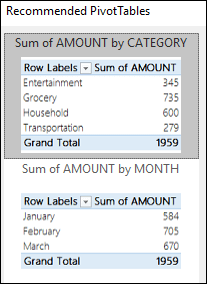
If you have limited experience with PivotTables, or are not sure how to get started, a Recommended PivotTable is a good choice. When you use this feature, Excel determines a meaningful layout by matching the data with the most suitable areas in the PivotTable. This helps give you a starting point for additional experimentation. After a recommended PivotTable is created, you can explore different orientations and rearrange fields to achieve your desired results. You can also download our interactive Make your first PivotTable tutorial.

1. Select a cell in the source data or table range.
2. Go to Insert >Recommended PivotTable.

1. Select a cell in the source data or table range.
2. Go to Insert >PivotTable.